Given the excitement around these methods, Chicago University has recently run the IGM Economic Experts Panel asking economic experts on whether the “ Randomized control trials are a valuable tool for making significant progress in poverty reduction”. The results of the poll are summarized in the graph below. 

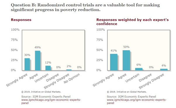
The chart above highlights respondents’ agreement distribution. What struck me most from the results was Angus Deaton’s strong disagreement with the statement – especially given that he is an expert in the field.

Why does Deaton strongly disagree? 

To answer that we would like to think about what the RCT is and how does it fit to answer the policy question. Let’s shed some light on it.

What is an RCT? 

RCT is a technique used predominantly in medical sciences, but also applied in economics quite intensively , especially in the last few decades. The technique works in the following way. Researchers randomly select a group of people to allocate them a clinical intervention (such as an anti-cancer pill). The comparison group (which is called the control group) is also randomly selected where they received a placebo intervention (such as a sugar pill). 

Then the researchers compare the difference between the groups to quantify the significance of the treatment (clinical intervention or “treatment effect”). 

In economic research, RCT is often applied in poverty alleviation schemes to help quantify the effect of the policy intervention. However, it has been applied much more widely giving insights about the labour market, behavioural economics, health economics, taxation, and industrial economics.

So an RCT tells me what a policy does? 

RCT gives us an empirical treatment effect given specific conditions. This is the type of thing economists will often call a stylised fact.

However, stylised facts cannot give us general policy effects – they tell us what the policy response was in a specific set of circumstances, but we need to be able to generalize that effect to apply it in other circumstances. 

This is where Deaton gets concerned, and where some of the push-back against RCT stems from. 

To get a policy effect we still need a model – simply scaling up an RCT involves imposing an implicit model about how the policy and behavioural responses work, one that assumes the scale of the policy change does not matter and that there are no general equilibrium effects.

This matters.  If we provided a minimum income payment in Treviso, Italy we may find certain changes in prices and labour supply responses in that community.  However, we could not then take that result and “scale it up” across Italy as a whole – as Treviso was not a closed system in the same way an entire country may be, and the larger scale of the policy would influence prices and labour market responses differently as a result (eg if a minimum income increased demand for particular goods, doing so in a small region may not change the price for that good – while doing it for the whole country would).

How economic models fit in here? 

Economic models provide the mechanism for generating generalisability.  At the same time, models and RCT results should work in a recipricotive way. 

Given the same conditions as the RCT, a good economic model should be able to replicate the result – or at least key attributes of it.  Given the ability to replicate an RCT for those conditions, the model then embeds key assumptions about why that result held and a description of the systems that make up the question at hand – this allows an economist to ask counterfactual questions about what would happen if the policy introduced was much larger.

However, it isn’t all one way. Models should in turn be reevaluated if a robust body of RCT evidence suggests that – for a given set of conditions – the models results are false.  RCTs provide the pieces of evidence that models should be able to replicate, while models provide a framework for understanding what can’t be measured and how other, counterfactual, policy changes will work.

Examples of policy implementations (treatments):

To clarify let’s talk about specific examples of how the RCT can be used. 

Minimum wage and labour market 

Let’s consider an example with minimum wage increase and the labour market outcomes. Card and Kruger (1993) found that the minimum wage increase in New Jersey led to employment increases in the state compared to the other state (Pennsylvania), where the same policy was not applied. 

Now if we want to take this result and generalise it to the population level, saying that if we increase minimum wage, it will lead to an increase in employment rate, we are making a mistake. Why? Because the same increase in the minimum wage in all states would have different impacts due to the composition of those states, the overall change in prices in the economy, and the capital structure and industries that are viable across the US economy.

However, it showed there were real shortcomings with models that could ONLY indicate that an increase in the minimum wage could reduce employment. This helped to generate a literature that has more carefully considered the role of minimum wages given the potential for market power and strategic interaction in the market for low wage workers. 

What is the solution then? 

In Deaton’s view too much is being asked of RCTs, and indeed people need to recognise how to “transport” the results to another context:

“More generally, demonstrating that a treatment works in one situation is exceedingly weak evidence that it will work in the same way elsewhere; this is the ‘transportation’ problem: what does it take to allow us to use the results in new contexts, whether policy contexts or in the development of theory?

It can only be addressed by using previous knowledge and understanding, i.e. by interpreting the RCT within some structure, the structure that, somewhat paradoxically, the RCT gets its credibility from refusing to use. If we want to go from an RCT to policy, we need to build a bridge from the RCT to the policy.”

Deaton’s concern, which is reasonable, is that RCTs are treated as a sole source of truth. But such a focus isn’t just misleading, it would be bad science.

Card and Kruger’s paper did not tell us that a higher minimum wage would increase employment – it taught us that reality is complicated, and the evaluation of policy must be based on trying to understand how this works, using both evidence and theory.  Duflo, Kremer, and Banerjee similarly see the importance of both – in her Economist as Plumber article Duflo notes:

“However, because the economist-plumber intervenes in the real world, she has a responsibility to assess the effects of whatever manipulation she was involved with, as rigorously as possible, and help correct the course: the economist-plumber needs to persistently experiment, and repeat the cycle of trying something out, observing, tinkering, trying again”

Deaton’s concern is that people will experiment and measure without ever trying to model and understand what they are doing – thereby generating a stream of published studies but no understanding.  Those that are more positive about the RCT revolution instead see such experimentation as part of this very iterative process that helps to describe the “transport” problem that Deaton is concerned about.

To sum it up 

Predicting a policy result from a given policy involves an implicit model – irrespective of the number of RCTs that have been run. However, these RCT provide a discipline that any worthwhile predictive model needs to be able to replicate – they provide the true stylised facts (if done properly) that a predictive model must match to be credible.

It’s not a long paper so click through and see how they did it.

HT: Marginal Revolution

Still, don’t read me.  Read Cochrane (here, here, here, here, here).  And Marginal Revolution (here, here, here, here, here, here).

Also I enjoyed this.  And this post on why the Chicago school gets so many Nobel laureates is a good counter-measure to all the arbitrary bile that can be thrown around on the interwebs .  I also enjoyed this post from Noah Smith.

I have a bias towards Shiller in all of this because of my interests.  He is a big proponent of trying to view economic phenomenon through a lens of history dependence (with the regulatory difficulties that entails) and has talked about how exciting neuroeconomics is – completely agree.  However, this has nothing to do with empirical finance in of itself, as this is not my field.  While I think some of the stuff is pretty cool (and remember really like GMM a few years back) I have nothing to say.  Hence why you should be going back and clicking those links to Cochrane and Marginal Revolution

The era in which an essayist can get away with ex cathedra pronouncements on factual questions in social science is coming to an end.

Very good, and Pinker’s co-operative version of science with the humanities seems appropriate to me (where instead we are merely asking about how to deal with certain propositions and using the best tools available).  I think Pinker won this debate, I am unsure why Wieseltier felt it necessary to take such an extreme position though – I think he initially believed Pinker was trying to force through a view based on the superiority of scientific authority (one that Pinker rules out in his initial article!), when he was really just suggesting the use of the scientific method (namely introducing a degree of the positivist view of theory creation) given the improvements in data availability and usability we have had.

As XKCD says:

But even within Pinker’s reasonable claims there is one area where I would be a touch careful – a direction I was hoping the debate would actually go in!   I would just caution being too confident about placing beliefs on the basis of ’empirical fact’.  We should definitely use the information and update our beliefs, but the Duhem-Quine thesis is even more binding in the social sciences than it is in the physical sciences – due to the lack of natural experiments and that more complicated causal chains involved.  [Note:  Would have also enjoyed a free will vs determinism debate]

Language and rhetoric allows us to give this context and give alternate hypotheses and elements of heterogeneity in society a fair go – even looking straight at empirical data, the use of these allows us to know what we can’t measure, helps establish a limit to the use of data, and helps us ‘pick’ what we should be trying to measure!  We should definitely make use of empirical data, and use it to establish underlying premises – but when it comes to writing an essay or op-ed the premise established from data could conceivably be so far in the background of the argument (due to the conditional nature of its use) that essayists may appear to be making ex cathedra pronouncements on issues that ‘on the surface’ appear to be factually false, but are actually appropriate.

Just to take the example in the piece, the 30-60% of Americans saying they take the bible literary (our fact) just tells us that this is what they reported to someone – it is not a revealed preference.  For this we need to see actual behaviour when making choice.  We could argue that they were saying this “to sound good to the interviewer” – even unconsciously.  Given this, the true number is well lower, and our view that literal views in religion are not widespread survives as a premise for whatever claim we are making.  In this way, the writer really has to appeal to authority – they do not have the space to write this out, but they have the argument around it in their backpocket.  Directly old auxiliary hypotheses!

I’d also note I really don’t know terribly much about these things, and it would make a lot more sense to find someone who works in an interdisciplinary field which already does this.  Someone who has a lot of experience with empirical data and models, but also write about language and works in a history focused type field.  Someone with an Economics History background.  The answer is pretty clear for the economists out there – Deirdre McCloskey.

Two quotes I’d like to note down here:

The more non-theoretical an empirical statistical problem is, the more randomization matters: control is pretty hard if one does not know what to control for

This reminded me of Mostly Harmless Econometrics, where the importance of randomization and natural experiments was drilled home throughout the book (for solving selection bias)

The difficult thing in subjects like economics/econometrics is that, for some questions we want to ask, we don’t actually get this type of data.  Given that, we are forced to add additional layers of theory and controls – an important point.  More generally, economics/econometrics also face up to other sources of endogeniety – and to be honest, some form of theory or structure is required to interpret those.  This is one way to view “theory” and “empirics” as essentially intertwined – we can’t really treat one well without also using the other, no matter how much we want to either abstract into a world of only data or only theory!

Furthermore:

Neyman-Pearson methodology in practice, finally, is vulnerable to data-mining, an abuse on which the different Neyman-Pearson papers do not comment.  It is implicitly assumed that the hypotheses are a priori given, but in many applications (certainly in the social sciences and econometrics) this assumption is not uniquely determined once the test is formulated after an analysis of the data.  Instead of falsification, this gives way to a verificationist approach disguised as Neyman-Pearson methodology.

I remember being told this in undergrad – data mining was bad, we needed an a priori model from theory before we tested.  This gave me quite a shock when I read Freakonomics.  Here was a book that seemed to accept, and enjoy data mining!  I was then taught VAR’s and seemingly told to over-fit a time series model massively.

Now to a degree this is cool – data is informing theory, as well as theory informing data.  As long as we view this as a process of Bayesian updating, and we make our statistic analysis replicable, there is a lot of positives here.

But we also have to be careful as noted here – actually here:

Now let us suppose that the investigators manipulate their design, analyses, and reporting so as to make more relationships cross the p = 0.05 threshold even though this would not have been crossed with a perfectly adhered to design and analysis and with perfect comprehensive reporting of the results, strictly according to the original study plan. Such manipulation could be done, for example, with serendipitous inclusion or exclusion of certain patients or controls, post hoc subgroup analyses, investigation of genetic contrasts that were not originally specified, changes in the disease or control definitions, and various combinations of selective or distorted reporting of the results. Commercially available “data mining” packages actually are proud of their ability to yield statistically significant results through data dredging. In the presence of bias with u = 0.10, the post-study probability that a research finding is true is only 4.4 × 10⁻⁴. Furthermore, even in the absence of any bias, when ten independent research teams perform similar experiments around the world, if one of them finds a formally statistically significant association, the probability that the research finding is true is only 1.5 × 10⁻⁴, hardly any higher than the probability we had before any of this extensive research was undertaken!

In my search for the appropriate XKCD cartoon to illustrate this I found this post that sums things up better than I do.

The same considerations apply when using significance tests in science: if you plan to do many such tests, you need to adjust for the fact that a “significant” result is more likely to occur by chance alone. (The R language has functions and packages for making such “multiple comparison” corrections.)

Now where does verificationism, and the use of Neyman-Pearson methodology fit into this? Well if practically we are acting as if all information comes from observation (which violates the implicit assumptions of N-P, but maybe not some of the practice), then the practice of data mining without doing proper meta-analysis, and with the fact that reported empirical results are a biased sample (biased towards rejecting the null), is particularly dangerous.

And if we carry on down that road, and build up a series of “estimates” to justify “social costs” on the basis of it – we may heavily overestimate true social costs no

Note:  Here I’m trying to interpret methodology things again, but I could of course be completely off track – critical comments are highly welcome

However, despite the great informational power of statistics, bear in mind that sample based statistics are still always measured with error.

How often do we hear news items that note something like: ‘according to the latest political poll, the support for the Haveigotadealforyou Party has increased from 9% to 9.5%” etc, but then just before closing the item they state that the survey has a 2% margin of error.

If you are awake to this point you suddenly realise that you have just been totally misled.

With an error margin of 2 percentage points, you cannot make any inference about anything within a 2 percentage point margin.

After discussing this point he states:

One can react to this article in (at least) two ways: one could become a bit more relaxed about the significance of changes reported in statistics or one could seek improvements to the accuracy of statistical collection.

In what areas do you think the first option is appropriate, and in what ways would it be worthwhile to increase spending to improve accuracy?

…with complex data series one can often hear patterns or persistent pitches that would be difficult to show visually. Musical pitches are periodic components of sound and repetition over time can be readily discerned by the listener.

Giles has previously covered the topic and it’s well worth having a look at the series he examines in that post. I know I’ve spent far too much time staring blankly at a volatile time series plot before attempting various transformations just so that my eyes can make sense of it. If there is a better way that uses other senses to quickly discern patterns in the data then I’m all for it!

For a more populist example, here’s a cellist playing a time series of temperature readings: A song of our warming planet

They take a panel of UK Competition Commission decisions from 1970–2003 and evaluate the effect of the chairman’s experience on the probability of an adverse finding. Using a panel of that size allows them to control for various effects such as the chairman’s age.

Using a unique data set of companies investigated under UK competition law, we find very strong experience effects for chairmen of investigation panels, estimated from the increase in experience of individual chairman. Probit and IV probit regressions indicate that replacing an inexperienced chairman with one of average experience increases the probability of a ‘guilty’ outcome by approximately 30% and, after chairing around 30 cases, a chairman is predicted to find almost every case guilty.

There is strong evidence that house prices and consumption are synchronised. There is, however, disagreement over the causes of this link. This study examines if there is a wealth effect of house prices on consumption. Using a household-level panel data set with information about house ownership, income, wealth and demographics for a large sample of the Danish population in the period 1987–96, we model the dependence of the growth rate of total household expenditure with unanticipated innovations to house prices. Controlling for factors related to competing explanations, we find little evidence of a housing wealth effect.

1. They are excellent writers,
2. They get to the point – and have a clear idea of how important this sort of issue is for trying to understand cyclical phenomenon,
3. They have pulled together a large data source consistently, which is a lot of work.

So as you can tell from that, I have a lot of respect for them, their work, and what they are doing.  However, I have a giant misgiving about the way they’ve framed the result they have found.  Fundamentally they HAVE NOT estimated the causal impact of housing wealth on retail sales/consumption.  In the introduction they do not make this claim hunting down an “association” … but by the conclusion this is what they are starting to claim they have done:

The importance of housing market wealth and financial wealth in affecting consumption is an empirical matter … we do find strong evidence that variations in housing market wealth have important effects upon consumption.

These descriptions are veering on causal, which is very inappropriate in a situation where you have an obvious, and likely significant, case of omitted variable bias!

Let us think about this.  Demand for housing is similar to demand for other durable goods – when confidence is high, unemployment is low, income expectations are elevated, and financial conditions are good, demand for both will rise, pushing up prices.  As a result there are some “third variables” that will drive up demand for both.  They cover this off at the end by stating:

Underlying our analysis is an assumption that it is useful to think of causality as running from wealth components to consumption, and not that, for example, the two are determined by some third variable, such as general confidence in the economy. We believe even more strongly that these new results demonstrate that it is useful to think of consumption as determined in accordance with the models we have presented. In consulting this evidence, recall that our measure of housing wealth excludes wealth changes due to changes in the size or quality of homes, changes that are likely to be correlated with consumption changes merely because housing services are a component of consumption. We have alluded elsewhere to others’ evidence using data on individuals that the reaction of consumption to stock market increases is stronger for stockholders than for non-stockholders (Mankiw and Zeldes, 1991), and that the reaction of consumption to housing price increases is stronger for homeowners than for renters. This lends additional credibility to our structural models when compared to a model that postulates that general confidence determines both consumption and asset prices.

To think about this point let’s think about housing.  Housing is a durable consumer good.  As the price of housing goes up relative to other goods and services, then given other goods and services constitute a “normal good”, spending on other goods and services should fall!  Of course, it also constitutes a transfer of wealth from homeowners to renters – and as a result, we have to ask about these separate markets in order to figure out what is going on.

As a result, the point that homeowners and renters behave differently is VERY useful, and justifies the study.  However, it in no way supports ignoring omitted variables and just deciding that the model is causal – in fact the way they have dismissed OVB is far too casual, given that there was no effort to deal with it (FE estimators deal with unobserved heterogeneity that is constant through time – this is not the case with our OV’s).

The evidence here appears to point at the fact that changes in house prices are a good proxy for changes in access to credit – hardly surprising given that housing is an asset and a durable consumer good.  When trying to understand the tendency of movements in retail spending, and the set of risks going forward for such spending, using house prices as a proxy for a set of “real structural” variables is useful.  However, this evidence is far from suggesting a causal relationship – and even further from suggesting that there is anything policy relevant here (as we need to understand the structure of the relationship in order to understand how changing policy settings will change outcomes – a change in policy settings can change the fundamental relationship between variables, think Lucas Critique!).

When the authors began to discuss this as causal, they should have stated that this provides an “upper bound” on the impact of housing wealth on consumption – and that more detailed analysis would be required.  They could even have gone further and stated that “given the size of the link, it is more likely that there is a tendency for higher house prices to drive up consumption” – that would have been mildly contentious, but reasonable.  As it is, their comments that they are estimating the size of a causal link are misleading.