Now I have no problem with breaking up monopolies, and I’m a huge fan of clear competition policy. But this isn’t going to deal with the “inflation” problem we are talking about. Let’s chat about it.
An earlier post here on “price controls” discusses a number of specific matters in more detail, but I think a higher level discussion would also be useful. To that end, I thought I’d share a twitter response I made to some bloke going on about corporate greed and inflation:
As you may have noticed in earlier posts, I haven’t given up on the transitory narrative (based on central banks managing expectations), but as Michael Reddell notes the outlook for this narrative does keep worsening:
I did your first year econ course, you said monopolists were price setters, so we need market power to get greed to influence prices – checkmate
Nice, and I hope you enjoyed the course. Sadly you are only remembering the words that we use, not the full nature of the content with that response – sometimes the way economists name things mean they can be misinterpreted.
A “price taking” firm only has the incentive to charge the market price – this does not mean they have to accept some fixed mark-up on cost, it means that market conditions determine the price they are incentivised to sell at!
If overall demand for a product rose, and we were looking at a product where new firms could not enter instantaneously, then this would lead to an increase in the market price – which would then be charged by our little competitive firms. They would earn supernormal profits which should, in time, lead to entry by other firms – this is what drives down the price again (if demand remains high). If there is uncertainty about future demand, then that acts as a additional cost for entry – which implies that higher demand may be met with higher profits in the case of perfect competition.
For a variety of market structures and levels of competition, higher demand would be expected to lead to higher prices and profits – the puzzle often was that, in the case of firms with market power, this was not the case! Instead, we would see their tacit collusion break down, leading to countercyclical margins and less price variability in situations with large oligopolistic firms.
So in other words, we do not need market power to get price and profit change when we have an increase in demand in the economy (relative to productive capacity) – and imperfect competition can actually reduce the relevance of this.
Now, in the current situation we have both significant fiscal spending (government demand) extremely low interest rates and a movement out of lockdown bring consumer spending into the current period (private demand) and disrupted supply chains for goods making the durable items and petrol that people are trying to buy more scarce.
In that situation, it would be good for people to delay purchases a bit – implying higher interest rates, and high prices (relative to future prices) serve that purpose.
But if they just didn’t lift prices there wouldn’t be inflation
No if prices never changed we would never have measured inflation – this also implies wages would never change as well mind.
But what would then happen is that when there is excessive demand the number of products would need to be rationed in some other way – lines, black market activity, empty shelves. Suddenly people that very much value a product would not find that it costs more – they would find that they can’t even buy it.
When demand is insufficient these fixed prices would imply that firms would see their stock building up, and without the ability to cut prices to clear stock they will simply produce much less – implying that larger layoffs and business failures would occur.
This is not to say that the current increase in demand may not propagate through prices in the way firms with market power behave. A clearly communicated “shock” that gives a firm the ability to wink and nod at other firms that it will “lift prices” may allow firms to collude, leading to price increases that would not have been possible with competition. This is the tacit collusion that we chatted about in the prior post, and a million other times here. And the empirical evidence tends to show that this does not occur usually during period of high demand.
And what about changes in relative prices – supply chain disruption is far from even across industry and product types, and so prices need to change to represent that scarcity. If there is less fuel available we want the price of fuel to be higher, so that those with a lower use value of that fuel self ration. Knowing that certain individuals may be in a vulnerable position to changes in fuel prices we may act to support their incomes, but not blunt that price signal.
Now monetary policy does aim to reduce the variability in prices – but it is doing so by reducing the variability in demand, not by telling prices to stay put.
Conclusion
Blaming the current increase in the price level, and the spectre of future inflation, on the greed of someone powerful achieves two things – it makes it a morality play, and it means that we think we can punish the “bad dudes” in order to solve the problem. But these things are not true.
Making a popular boogey man might be good politics – but it doesn’t help the wellbeing of a nations citizens. As Chris Conlon says:
For those who don’t like videos, there is a transcript below.
[Matt]
Gulnara has told me I need to get a haircut.
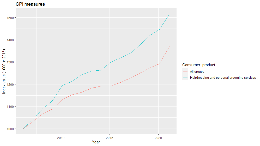
I’ve selected the place I’m going to go due to their good and reliable service. But something I did notice is that, everywhere I looked, the cost of a haircut is a lot higher than when I was young.
Now there has been inflation – or a general increase in prices – during that time. But this doesn’t quite cover it. Looking at the CPI category for personal care – which includes haircuts – the prices have gone up 52% between 2006 and 2021 while the average price of consumer goods as a whole has risen 37%.
So to solve this puzzle I thought I’d call out to my favourite economist to see what she has to say.
[Gulnara]
We have all seen this graph from the United States [Vox graph]. This shows that the issue Matt is chatting about isn’t just about his haircuts – which are necessary by the way – but also refers to a wide range of different products.
Payments for services, such as college fees and medical care stand out as items that have become relatively more expensive.
Meanwhile durable goods, such as cars, furniture, and toys have become relatively cheaper.
As the economy has matured and grown, different needs and wants have been met, making room for different avenues for scarcity.
Growing global trade, along with technological progress, has helped to increase productivity across a range of sectors. However, even those sectors that have not seen productivity rise – and who have not seen relative demand change – have been influenced by this, due to the interrelationship between industries.
No matter how much we look at different sectors and industries separately, they are all bound together by a complex web of related demand for inputs – especially through shared labour and capital markets. And it is only by considering those that we can think about Matt’s haircut.
However, answering Matt’s question doesn’t just tell us about haircuts – and it doesn’t just tell us about long-run economic history and economic development – it also helps us to understand some of the things going on, right now, in the COVID afflicted global environment.
As a result, understanding Matt’s haircut might help us to think about the risks and opportunities of the post-pandemic economy.
So let’s get this started.
Baumol effect
In the 1960s economists noticed something funny going on with the price of different things. The 1966 paper “Performing Arts, The Economic Dilemma: a study of problems common to theater, opera, music, and dance” by Baumol and Bowen looked at this issue specifically with a Beethoven String Quartet.
Now we can all understand the beauty and value of listening to a rendition of Moonlight Sonata. And seeing such a show live is a beautiful thing.
In fact, let’s play a bit of Fur Elise.
Enough of that, back to economics.
The quality and quantity of such performances has not really changed through time – there has been no productivity improvements in the provision of Moonlight Sonata performances.
And yet, the salary of a musical performer is now higher than it was in the time of Beethoven – in fact salaries keep rising each year (An Updated Look At Top-Tier Musician Compensation 2016 – Adaptistration).
If productivity is not rising in the classical music performance sector, why are wages rising? The key point here is that individuals have skills that are transferable between jobs – which means they can perform different tasks in jobs across the labour market. Although it is unlikely that a Cello player would go into a car factory to play cello, they would have skills to undertake some of the tasks within the factory – and could be trained on the job to do others.
As a result, if the Cello player only received the same wage as someone in the 19th century it is likely they would decide to work elsewhere – such as in the car factory where productivity has increased markedly.
Here the ability to automate, innovate, or increase the amount of capital in “capital intensive” sectors such as the car factory, helps to boost labour productivity. Meanwhile the labour intensive “productivity fixed” nature of the orchestra does not see labour productivity rise for that job.
Wages will rise in sectors where labour productivity rises. This increase in wages will lead to upward pressure in other sectors, pushing up wages even though the labour productivity in that sector has not risen. This will in turn force firms to shut down or to increase prices – and if consumers armed with higher wages were willing to bear those prices, we could well end up in a situation where we are now. A situation with musical performances continuing, but at a higher price and with higher wages paid.
Baumol cost “disease” refers to the Vox graph we noted earlier – it is the application of the Baumol effect to prices. However, the disease makes it sound like these higher prices are fundamentally a bad thing. You will hear “we used to make these things more cheaply, why can’t we now!” or “it gets made so much more cheaply overseas”. Well if it was just due to the Baumol effect, it is because the average wage rate in the economy is higher because average productivity is higher!
This is not to say there can’t be regulatory or competition related barriers that create issues. But rising prices and wages in these “fixed productivity” sectors that are reliant on labour intensive work can just be a product of everyone benefiting from growing productivity – hardly a disease at all.
[Matt]
Balassa-Samuelson
Thanks Gulnara.
On top of this, in the 1960s some macroeconomists you may have heard of – Bela Balassa and Paul Samuleson – were interested in why consumer prices tend to be higher in countries that have high average incomes, an empirical regularity that is termed the Penn Effect.
In this instance the puzzle exists because of the law of one price – the idea that in a world with open and free trade, consumer prices should be driven down to the same level across countries.
However, this need not occur, as it is costly to transport certain goods and services across borders. Specifically, we may view some goods as “tradable” because the transport cost is sufficiently low while other goods and services are “non-tradable” because these transportation costs are high. My potential haircut is an example of a non-tradable product, where getting a haircut in the United States would involve quite a significant amount of time and expense unrelated to the act of cutting the hair itself!
The law of one price would suggest that prices are only driven down in relation to the transportation cost – and so there should be more convergence in prices between tradable products than there is for non-tradable products.
Rising trade and increasing productivity in tradable sectors have helped to push a convergence in global prices for tradable products – and have also generated productivity increases, and in some circumstances terms of trade increases, for a variety of trading countries. Increasing tradable sector productivity has then resulted in rising output and incomes across the world.
But how are non-tradable prices determined? At face value non-tradable prices are determined by local demand for the product. So if average incomes rise, due to an increase in productivity of the tradable sector, there may be increased demand for these local products which will bid up their prices.
However, as was the case with my haircut or the music discussed above, demand can only take us so far. If there is domestic competition then, even though people’s willingness to pay in the tradable sector is higher, entry to the market will see prices decline to their prior level.
Instead, the key driver of the Balassa-Samuelson effect is the Baumol effect and wages. An increase in productivity in the tradable sector translates into higher wages. Higher wages in that sector give individuals who are working in the non-tradable sector an incentive to change their jobs – driving up the wage rate in the non-tradable sector. The higher costs in the non-tradable sector are then passed on in higher prices.
In 1989 Rudiger Dornbusch took this a step further and noted that the nature of demand changed as countries become wealthier, with demand for services increasing disproportionately EconPapers: Purchasing Power Parity (repec.org). Such an income effect can further reinforce these changes, and reinforces the way tradable sector productivity shocks are distributed across an economy.
Combined with the Balassa-Samuelson effect, this Dornbusch result tells us that income gains associated with increases in tradable sector productivity may be weaker than suggested by GDP comparisons at market exchange rates. However, it also indicates that such gains are distributed much more widely across the economy, rather than just where the productivity increase occurs.
This can be seen in prices – as shown on this tweet. Durable goods – which by definition are things that can be stored and so are usually tradable – have not grown in price as quickly as services for a long period of time. That is until the pandemic hit, pushing up effective transportation costs!
With parts of the service sector becoming increasingly “tradable”, the Dornbusch result of rising demand for services may also not remain a driver of the Penn effect going forward – if my income goes up I do not buy more haircuts, but I might buy more subscriptions to news services. In that way, increasing divergence between tradable and non-tradable prices and their relative productivities will need to be due to the Balassa-Samuelson effect itself.
So how does this relate to Matt’s haircut? [Conclusion]
Pulling these ideas together, we have not seen great technological innovation in the type of haircut, Matt gets over his long life. But we have seen innovations and productivity increases in tradable products, with greater productivity in New Zealand exports as well as higher relative prices received for those exports.
The productivity lift implies that there is more income overall, and part of this income is then allocated to those providing haircuts! As a result, the lift in haircut prices is a sign of growing productivity in other parts of the economy.
It could be that there are other drivers – namely regulation or competition – but such a change could also be a symptom of a healthy economy. Rather than a disease that we need to do something about, it is just a natural sharing of the benefits of growth.
So let’s go get Matt this haircut, and we’ll see you again next time. Byeee!
]]>For those who don’t want to listen to a video, we’ve popped the script below.
We’ve chatted about why we care about GDP and the different ways of measuring it – be it through expenditure on final items, the value-added in each industry, or the income paid to those providing a “factor of production” such as work time or capital equipment.
In these chats we established that however we measure it, these measures of “expenditure” “production” and “income” all give us the same result for GDP – and this tells us that the amount we produce, the amount we consume, and the amount of income we have are really all the same thing.
This is a powerful result that has been used to say “Supply creates its own demand” or, as the bloke on my t-shirt says, that “demand creates its own supply”. Behind all of this we always need to model a process to truly understand how the macroeconomy works and what trade-offs there are.
[Gulnara]
However, out of context this result is also misleading – and can lead us to get the wrong impression about how society is progressing or the opportunities available to people. Even ignoring other attributes that economists like to add in – the distribution of income, environmental change, and non-monetary value stemming from your interaction with your community – this perspective can miss important things even in terms of our narrow understanding of monetary incomes.
In this video we are going to think a little bit about that, and see what other measures we can look at from the national accounts that may give us a wider perspective on incomes.
GDP and income
[Back to Matt]
As we noted in a prior video, GDP can be measured by taking all expenditure on final items, taking all income paid to labour, capital, and through indirect taxes, or by calculating the value added in each industry and adding them up. And each of these measures will give us the same number!
This measure is amazing at helping us understand the use of society’s scarce factors of production, gives us an insight into economic progress in a country, allows us to understand and compare production and incomes between countries, and provides a useful piece of information for asking about policy trade-offs when we use it with economic models.
However, when it comes to cross-country and time based comparisons we immediately run into an issue – prices change through time, and different countries use different currencies.
If we are looking at one country or countries with the same currency everything is in the same “unit of account” which makes it easy to add up – but how do we add up a New Zealand dollar and a Japanese Yen for building a GDP measure?
When comparing across countries we need to adjust for the fact that different units of the currency can be exchanged for the same goods. We can’t just use exchange rates here as they don’t give us the full picture due to non-tradable goods and services. Furthermore,these exchange rates can be excessively volatile and as assets currencies may be valued for reasons other than the strict ability to purchase goods and services.
We aren’t going to focus on cross-country comparisons and therefore those types of measures right now, but will cover it in a future video.
Our focus here will be on the time based dimension. We know that a New Zealand dollar today cannot buy the same number of chocolate bars as a New Zealand dollar could when I was a kid – sadly. As a result, if we construct GDP just by counting the number of dollars spent on these items, then when comparing GDP numbers over time we will end up with a measure that captures both the increase in the price of goods and services as well as an increase in the actual number of them.
The measure that takes “current prices” to calculate GDP – the equivalent of just adding up the number of dollars spent – is called nominal GDP. While the measure that adjusts for the fact that prices changed and attempts to measure the volume of GDP over time is called real GDP.
Getting from nominal to real GDP involves figuring out a way to remove the price effect, or what is termed deflating nominal GDP for price growth. The GDP deflator captures the aggregate price effect through time, and by dividing nominal GDP by this deflator we get our measure of real GDP.
As we often care about the amount of stuff available to buy, rather than the number of New Zealand dollars floating around to spend on it, real GDP is normally the measure we are talking about when we talk about GDP as income. However, both measures are useful and have their place for asking different questions.
To give this all a bit of context, let’s pull up the data and look at these measures for New Zealand.
[R session]
Here we have pulled some data off the Stats NZ website and made some quick and nasty graphs. This first one shows us New Zealand GDP in nominal and real terms between 2000 and 2020.

Note how nominal GDP starts below real GDP and then climbs above it. What does this mean? Well it means the nominal GDP was growing faster than real GDP, which is what we would expect given that prices were rising!
Furthermore, they are equal during 2009 – implying that we are deflating nominal GDP to get real GDP in 2009 prices.
This is the income of the nation, but as we are looking at incomes we might want to know about the incomes per person – or per capita. As populations are growing that looks like a second graph here.
This shows a similar trend, but you will notice that the lines are a bit flatter (or that the Y-axis increases by a smaller proportion). This is because the population was growing during this period, so part of the increase in GDP was associated with there simply being more people.
The real GDP per capita number tells us that, in New Zealand borders, significantly more output is created per person was created in 2020 than was the case in 2000 – 38% more to be precise! This opens up a world of questions, are we using more inputs (i.e. working more, using more environmental capital, building up more physical capital) or have we just learned how to use what we have in a more efficient way – what is called multifactor productivity growth.
But we aren’t answering those here. Instead we want to ask, is this income? Over to you Gully.
What is macroeconomic “income”
[Gulnara]
Thanks again Matt.
Describing GDP and income in the way above is typical for an introductory economics course, and feels very natural. However, it is also misleading. To truly think about income we need to ask what income actually is.
In Hicks 1946, John Hicks stated that income was “the maximum value which [a man] can consume during a week, and still expect to be as well off at the end of the week as he was in the beginning.”. As one of the founders of the post-war “neo-classical synthesis”, and as a famous welfare economist, it is this definition of income that captures what an economist is thinking about when they say “income”.
It is then the equivalence between consumption + savings (potential consumption) and production at the macro level that leads us to view income as essentially GDP.
Income in this economist’s world is “potential consumption”, as it is this ability to consume final goods and services through time that generates wellbeing and welfare.
GDP on the other hand is a measure of the use of factors of production to generate value added/output – the rationale for looking at this is to understand the utilisation of factors of production, especially workers, in market activities. As noted by Matt above, the focus is also on the number of items.
In this way, much of GDP is the act of creating some value associated with a final product that is consumed – but there may be cases where the factor of production is instead used in order to “maintain how well off they are” or where the residence of the individual who claims the output differs from the residence of the factors of production. These differences will lead to a gap between our true concept of income and GDP – so let’s talk about them a bit more.
Maintaining assets
[Matt]
Thanks Gulnara. The issue I want to talk about a bit more is that of maintenance.
The “gross” in gross domestic product refers to the fact that ALL investment is included in the measure.
If you own a building and you use it to run a business then that refers to a capital item. You may invest in that building by adding an extra floor, improving the air conditioning with services like www.newcastleairconditioning.co.uk, painting the building, or replacing the showers. All this investment activity will be measured at once – however, some part of it refers to maintaining the productive use of the asset while some refers to increasing the productive use of the asset.
Why would we need to maintain anything? Well, time takes its toll on all of us – especially capital assets. This depreciation in the usefulness of the capital item is sometimes called “consumption of fixed capital”, and GDP includes investment that is solely about keeping the capital item as productive as it was before.
However, if we imagined someone producing something for themselves the decision to repair something doesn’t constitute a new thing for them to consume – so we wouldn’t view it as part of their “income” or an increase in their ability to consume while maintaining their current position. Instead, this is an expense that is required to keep themselves in that position!
The measure that tries to adjust for this given estimates of depreciation and measures of the capital stock is Net Domestic Product.
[R session]
We will construct Net Domestic Product from the Stats NZ data and graph it here as well. For this we have subtracted the Stats NZ estimate of “consumption of fixed capital” from GDP, and then used the same deflator to work out a real value. True Net Domestic Product will look a little bit different, but this gets us close enough to chat about.

So what is this graph showing?
Net Domestic Product moves in a similar way to GDP, but is lower. This makes sense as we are subtracting an “expense” that isn’t included in GDP. By taking away the part of GDP that needs to be used to maintain capital equipment we have a more genuine measure of income relative to the definition Gulnara gave above.
This figure grew by 37.7% – slightly less than the growth in GDP over the same period. Why is it different? If the capital stock per person has risen, or the types of assets we hold depreciate more quickly – such as computers – then the amount of maintenance that needs to be paid will rise. As a result, Net Domestic Product growing by less is also consistent with the changing nature of the economy over the past 20 years.
Opening the borders
[Gulnara]
Things become more complex when we open ourselves up to the rest of the world.
Three things happen when we admit there are other countries:
- Domestic residents can own assets overseas, and so are able to consume things that are produced overseas – similarly foreign residents can own domestic assets, giving them a claim on some of this domestic production that is measured by GDP.
- Domestic products might be sold overseas (exports), and foreign products may be purchased and consumed domestically (imports). Imports are part of consumption, and must be funded to some degree by exports. If the relative price of exports and imports increases , domestic residents can now consume more for the same amount of production.
- Transfers, such as charitable giving and intermittences, involves residents in one country sacrificing consumption to provide those opportunities to others overseas.
In this way, GDP remains as a measure of what is “produced” within a country – it measures what is made with factors of production within national boundaries. But this does not immediately mean that it reflects the claim on products for people who live within those borders!
Gross National Product or GNP is the measure that attempts to adjust for the income of domestic residents overseas, and the income of foreign residents that is generated in the domestic economy. This is very similar to Gross National Income, or GNI – conceptually they should be the same, but in some accounts the residency definition or definition of primary income (income from factors of production) that are included can vary between the two.
However, secondary income (such as the intermittences noted above) are missing in these measures. Adding in net transfers from above provides a measure termed GNDI (gross national disposable income) as an aggregate income measure. By capturing all foreign transactions, the construction of this measure also captures changes in the terms of trade as “income” – in a way that GDP does not. (isi_box1_jun_2015.pdf (banrep.gov.co))
Taking GNDI, we run into the same issue that Matt talked about above – there is some investment that is just about maintaining the stock of capital. Subtracting this depreciation then leaves us with two other measures that you may hear about, NNI or Net National Income, and NNDI or Net National Disposable Income.
Do all of these adjustments change much? Let’s look at the New Zealand data with Matt!
[Matt on R part and summing up]
For these figures we are going to stick with the nominal data provided by Stats NZ. This is because real figures are not provided, and trying to back out the appropriate price deflators for these different indices will take a bit of time without necessarily adding much value.
With that out of the way, let’s plot everything from the Stats NZ experimental national accounts.

As we can see here there are potentially a few data issues in this experimental series – so I want us to focus on the relativities rather than the individual series shape over time.
GDP is at the top, with GNI and GDI catching up through time. GNI and GNDI are also very close to each other. NDI is then significantly lower than the others – which does make sense.
So why is GNI below GDI in New Zealand? Remember that we get from one to the other by subtracting the domestic production that is claimed by foreign residents and adding in foreign production that is claimed or owned by New Zealand residents. New Zealand on average borrows from the rest of the world, and it is the income flows associated with this that explains the gap!
However, the deflator does matter when we want to think about the key differences between GNDI and GDP – namely changes in the relative price of exports and imports, or the terms of trade. For this we do want to consider how real measures may look different solely on this basis.

Here we get a much sharper change in the relative value of GDP and GNDI than when we looked at the nominal values. Why is that? In this instance New Zealand has seen a very substantial increase in its terms of trade – or the price of exports relative to the price of imports – over this period. When we deflate the two income series, that terms of trade difference shows up as another part of the change in these measures.
Between 1992 and 2021 real GDP per capita rose 58% while real GNDI per capita rose 77% – as a result this is a very significant difference. So how do we think about which income measure to use?
The fact that New Zealand can now buy a lot more imports from the exports it sells is an increase in income in the GNDI sense – and it is not captured directly by real GDP. How does this work? If exports remained fixed and more imports were purchased for consumers to consume, then both C and M would increase in the GDP equation – cancelling each other out.
However, this is real income – having people overseas give New Zealanders more products for the same exports is exactly the same as exports becoming more productive in terms of the amount of goods and services available for New Zealanders to use. As a result, understanding this change is extremely important!
Conclusion
As we’ve noted above, looking at national accounts to get an idea of material wellbeing can be complex – and MOTU has been undertaking work trying to get a more detailed understanding of this in recent years: Motu-Note-21-Material-Wellbeing-of-NZ-Households.pdf
However, by clearly articulating what GDP is, and how it may measure some things we don’t truly see as “income or potential consumption” we’ve been able to work out some alternative measures that already exist in the data to chat about what is happening.
These measures give us additional information which may change the way we see New Zealand’s productivity performance, inequality within the country, New Zealand’s wealth and income relative to other countries and a multitude of other narratives that are given in the media and common discussion. However, we’ll leave it here and we would be eager to hear if this perspective is useful in helping you understand a little more about our beautiful little island.
]]>
The increase in prices in the US over the past year has been generating considerable angst – and comments that “price controls are needed to deal with inflation, due to corporate greed”. This has led to lots of people saying things on Twitter, with individuals who different people may see as authorities taking very different views on the topic:
How about we step back from the name calling to try to think about what these terms mean and what people are saying – as in the end it is likely people are talking a little bit past each other, and when that happens the rest of us can just get confused!
Are we talking about inflation?
To start with, is what we are observing at the moment “inflation”? This is a point that often gets missed, but it is essential to understanding the distinction between different points of view.
In the United States (where a lot of this discussion is ongoing), the consumer price index has increased by 6.8% between November 2020 and November 2021. There are three things happening here that give us our general context:
- A relative surge in demand for goods while demand for services is more mild
- Supply chain disruption
- Relatively higher price growth in the US than in other countries.
The increase in prices occurred in the face of post-pandemic supply chain disruption and significant fiscal and monetary stimulus – which has supported consumer demand. With some degree of nervousness about using public facing services, relative demand for goods is at an all time high – and so the already interrupted supply chains into and around the US are struggling.
Given a shortage of goods the increase in demand has translated into higher prices – a mechanism that is common for any type of rationing.
Furthermore, looking through the price categories, pricing pressures exist all across the set of goods and services for sale – yes energy and used car prices have risen by more, but price increases appear to be quite widespread.
This tells us that there has been a generalised increase in prices rather than just an increase “specific key sectors” as the article suggests. So this indicates that there is likely something increasing “all prices” rather than just the selected prices the article suggests targeting.
Furthermore, the lift in the US is higher than other countries have experienced – suggesting that there is an element of this that is US specific:
So that general lift is inflation right? Well not necessarily – and that is where everyone has been a bit slack. Inflation is “persistent growth in the level of prices”. If the supply chain interruption is temporary then this is a one-off price level change – which isn’t what we normally think of when talking about “inflation”.
This distinction often gets muddied as we care about the change in our ability to purchase goods and services – but the distinction is central if we are to think about the nature and role of monetary policy.
You may have heard of team transitory who are the individuals who believe it is supply chain interruption that is the primary cause of higher prices. This team does not anticipate future inflation once supply chains begin to function “normally” and in that context, a period of weaker price growth would be likely in the future once that occurs.
However, Elizabeth Warren recently took part of team transitory in another direction – by pointing out that measures of corporate profitability have increased. How is this relevant – we will get back to this soon I promise – but for now just remember that the view of imposing price controls is partially from this team.
Furthermore, even those in team transitory that do not believe in price controls are more sympathetic to leaving monetary conditions stimulatory (i.e. bond purchases and lower interest rates) and further government borrowing and stimulus payments. Why – because it is a temporary supply shock that has pushed up prices, and so allowing higher prices temporarily to prevent a decline in output/unemployment is seen as appropriate. At the very start of COVID, this was consistent with how Gulnara described the role of monetary policy in the face of such a shock – and a related lift in prices due to the Fed looking through supply chain disruption can be seen as consistent and reasonable.
A supply shock reduces income, and looking through the shock and allowing a one-off increase in prices (as opposed to trying to reduce demand to bring prices down) is seen as a fair way of distributing the shock – at least as far as monetary authorities are responsible for such things.
There is a different team of economists out there who see matters quite differently. Noting that the quantity of goods sold far exceeds anything seen in the past, this group views the focus on “supply chain disruption” as overstated – instead supply chains are overwhelmed because there is excessive demand. I see the article uses “team stagnation” which is a dumb name trying to discredit the idea – it is “team permanent”.
If monetary and fiscal conditions remain expansionary in the face of excessive demand, then prices will continue to grow – leading to expectations of future price growth among individuals and firms. These expectations then filter into price and wage setting behaviour, and become self-fulfilling – generating persistent growth in all prices. This is inflation.
The feather in team permanents hat is the differential change in inflationary pressures in the US relative to other “similar” countries. If prices are rising more quickly in the US than in other countries with similar supply chain disruption, then the additional price increase may well be due to greater domestic demand – and may be expected to persist generating true inflation and higher inflation expectations.
To this group a portion of the current increase in prices is inflation – as it is the start of a persistent process of rising prices.
Price controls, margins, and the price level
If we are experiencing genuine inflation then price controls are, to be frank, an incredibly dumb suggestion. Even when Tobin spoke in favour of such controls in 1981 (Economist Tobin on Inflation: How It Started, How to Stop It – The Washington Post) this was based on the view that it was not excessive demand generating the inflation – but the interruption of the oil price shocks.
<iframe src=’https://d3fy651gv2fhd3.cloudfront.net/embed/?s=cpi+yoy&v=202112101416V20200908&d1=19700103&d2=20220103&h=300&w=600′ height=’300′ width=’600′ frameborder=’0′ scrolling=’no’></iframe><br />source: <a href=’https://tradingeconomics.com/united-states/inflation-cpi‘>tradingeconomics.com</a>
There is a point here. Both of the teams noted above agree that the underlying supply shocks have consequently reduced incomes – and that higher prices are a part of determining who bears the reduction in “productivity” in some sense due to this shock.
A desire to then “control prices” is a wish to avoid the current distributional consequences. However, it is not costless.
If prices are not allowed to rise to ration the increase in demand, then something else will have to give – fewer goods and services will be available, the relative price anything without a rationed price (i.e. black market sales) will change, the intervention will create uncertainty about voluntary exchange, and finally once the controls are removed prices will simply rebound. The suggestion that selected prices are frozen is especially disconcerting as it will incentivise firms trying to reclassify products out of scope and lead to pricing pressure leaking out to other products while these products are arbitrarily rationed.
Contrary to the related articles that appear to suggest this isn’t true, we have endless examples of this occurred across the world – Venezuela, Argentina, the United States through the 1970s, New Zealand under Muldoon with freezes occurring between 1976 and 1984 (The wage and price freeze, 1982–1984 – Law and the economy – Te Ara Encyclopedia of New Zealand).
If instead we are viewing this as a one-off price change, then is the argument different?
If it was, it wouldn’t be the argument in the article linked above – which seemed to ignore the rationing that occurred for years following WWII as a natural part of the same issue, where the supply chain was shifting from significant central direction (to produce war equipment) to the private provision of consumer goods. The supply chain in the current situation has not had to change what it produced, or have been destroyed by a disaster, it is instead struggling under a mixture of higher costs and high demand.
Higher prices are the rationing mechanism at play given where the balance of supply and demand is – if we fix prices de facto lower the quantity of purchases further, then some individuals who value the goods at a very high price now would not be able to receive them. So far, no rationale. Furthermore, as the suggestion is to target specific “selected prices” – this will lead to increased demand for substitute products, leading to the pricing pressure leaking to other items. Given the rationale of targeting products who experience a price increase this is likely to lead to a poorly timed game of whack-a-mole with prices, all while the proximate cause of inflation – excessive aggregate demand – is ignored.
Such price fixing exacerbates the issue at hand – which is that households cannot get the goods and services they want given their real incomes. If instead of fixing prices we ensure that underlying fiscal policy is appropriately set to set a floor on individuals incomes, and that competitive issues are sufficiently dealt with to allow individuals to have sufficient power when they consume or go to work, then the distributional consequences are likely to be less severe.
If it is demand that is driving up prices, then the rationing functions over time – the high prices now push people who can wait to delay purchases, internalising the fact that supply chains are currently struggling. If prices do not reflect that, then in a rationed environment such products start to be allocated on the basis of luck and other forms of power – it will not reverse out the supply shock, and for some who complain goods are two expensive now it will simply make the goods unavailable.
Power dynamics and corporate profit
The concern about power dynamics is highlighted by the focus on corporate profit and “price gouging”. The idea here may be that producers are using this as a way to collude on higher prices and margins. As a result, there may be a way to undermine this collusion and increase quantity and reduce prices – solely benefiting households.
Now this is likely not an argument about monopoly or heavy concentration itself. The argument that a monopoly is taking this as an opportunity to charge customers more has to contend with the counter argument – if they could normally charge customers more why don’t they? Arguments that rely on “gouging” need to explain why this gouging doesn’t normally occur, and if it is a result of current scarcity why the price signal itself isn’t appropriate – after all, not having access to the product is the same as it having an infinite price to the consumer.
If the argument is just that demand is “currently high” then how is that different to stating that we should reduce aggregate demand which is what team permanent is saying? There is a distinction between their being demand for a specific product due to a crisis – and there being general high demand. And this article appears to confuse the two.
To try to make the best argument for this view about price fixing we need a coordination issue, we need some idea of oligopolistic firms and price setting.
The Green and Porter (1984) model of price setting among oligopolists may give us a solution here – during states of “high demand” oligopolists may collude and hold up profits, but when general demand falls they are unsure if they are being betrayed or if the economy is slowing. Given this they are more likely to “punish” by cutting prices when the economy slows. Here we have clear information of a “high demand” state, and so firms have agreed to collude.
The issue with this model is that is just doesn’t fit the data – rather than being pro-cyclical prices are often found to be counter-cyclical (i.e. Why Don’t Prices Rise During Periods of Peak Demand? Evidence from Scanner Data – American Economic Association (aeaweb.org)).
This result isn’t just in the annals of economic estimates – it is something you can see all the time by going to the supermarket. I’ve seen it for Nurofen (Why do supermarkets cut the price of medicine when people are getting ill? – TVHE), during COVID I saw it for toilet paper (Understanding Wellington and toilet paper – TVHE). Why?
That is where an alternative theory comes in, Rotemberg and Saloner (1986). If there are “high” demand and “low” demand states then the benefit associated with defecting from collusion is greater when demand is high – as a result, when demand is high and people are fully informed it is high, a price war and lower profitability is likely.
So why are corporate profits high, if our view of an observable demand shock would lead to lower profitability?
One way to do this would be to go back to view this predominantly as a supply shock rather than a demand shock, implying that post-COVID can be viewed as a low demand state. But that just isn’t consistent with the evidence relating to the quantity of goods being sold.
And that tells me that this IS an interesting puzzle – it isn’t about inflation itself, it is about the magnitude of the increase in corporate profits coming out of a pandemic during a period of elevated demand.
When I see a puzzle the first thing I want to do is look at the data more carefully.
Profit and the national accounts
In such a case the first thing I’d want to look at is what the data is – we are being told this is profit, but I know that national accounts don’t always match up with what we think. The key item I see here that interests me is the “Expenses exclude deductions for bad debt, depletion, and amortization“ – so bad debts that were written off, and assets and stock that was lost, are not included in expenses … and so form part of profit!
Inventory valuation adjustment (the IVA mentioned in the profits title) should have captured the majority of this loss as shown in the IVA figures:

Corporate Inventory Valuation Adjustment (CIVA) | FRED | St. Louis Fed (stlouisfed.org)
However, such revaluations tend to be fairly conservative. When combined with non-inventory write-offs in the period, this suggests that some of the increase in profit will only represent these costs to the business. As these are largely fixed costs we may still be surprised that firms have passed them on – however, if the costs were necessary to crystalise in order to being operating in a post-lockdown environment and businesses were liquidity constrained such pass-through may seem plausible.
Furthermore, if the current environment is very risky businesses may be unwilling to take on investment unless they are sufficiently rewarded for taking on the risk of their investment being sunk – which would also lead to higher profit levels.
A disaster that interrupted supply chains and destroyed inventories, and in the aftermath saw corporate profit rise when such losses are not recognised feels as if a major cost and risk parts of the cost shock is not being counted in the corporate profit figures. In an uncertain environment firms will want certainty about cash-flow, and will want to hold liquid assets in case they are faced with another shock – exactly the same way households function in such an uncertain environment.
Now it is useful to ask what else we would see in the data if this was an explanation. We would expect dividends to not change, while undistributed income and net private savings surges – as the undistributed income is essentially “invested” to pay for the costs noted above. Sure enough, this is exactly how the data looks:

Net private saving: Domestic business (A127RC1Q027SBEA) | FRED | St. Louis Fed (stlouisfed.org)

However, this does tell us that corporate firms were able to pass on these costs – which itself suggests that there is more going on. To understand this further we need to recognise that it is a bit strange to focus only on corporate profits and not the income of other capital and labour owners. So let’s take a look at that.


From September 2019 (pre-COVID) corporate profits have risen 29%. Over the same period compensation of employees rose 12%. These are all in current prices (Q3 2021, Table 1.14. Gross Value Added of Domestic Corporate Business in Current Dollars and Gross Value Added of Nonfinancial Domestic Corporate Business in Current and Chained Dollars: Quarterly | FRED | St. Louis Fed (stlouisfed.org)). With all incomes increasing and limited capacity to make goods and services this sounds a lot like a general “demand” shock driving up prices – a focus on only one income measure was hiding that!
The 17% percentage point gap between corporate profit growth and compensation of employee growth could plausibly be explained by increased risk in the trading environment, and “missed costs on business” in the national accounts figures that are being investigated. In this way, when we look at all the numbers as a whole it looks like a smaller puzzle – and more like there is a surge in domestic demand in the United States.
Ok why do I care
The distinction between this being a “supply shock” and a “demand shock” matters for what we would see as appropriate central bank action. If there is truly excess demand then tighter conditions are warranted – if it is mainly about supply disruption and a “price level shock” then there is less need for tighter monetary policy, and more of a need to communicate to manage inflation expectations.
Working through the data, the higher level of corporate profitability – and all incomes – makes the argument that this is a demand shock relatively stronger, rather than weaker. The argument given for price freezes does not support price freezes, but instead supports the tightening of monetary and fiscal policy the author says is inappropriate.
This is the key with economics – the author recognises this but there are other, unsaid, arguments in the background.
It appears the author is pushing for price freezes believes that there should be more government spending and investment in specific sectors, that the size of government should be larger, and that more resources should be directed by the state – and this is a legitimate position that they can take, and a legitimate position for people to strongly agree or disagree with. They are not thinking about inflation vs no inflation, but are instead worried about the political economy associated with reducing demand – and it occurring through reduced government spending.
In this world underlying “true” inflation is a tax, and this is a politically expedient way to have a greater tax burden to fund underlying expenditure. I would prefer the author was instead transparent and stated that they want more spending and taxation, rather than arbitrary calls to freeze prices based on corporate greed – but by obfuscating trade-offs they may feel that the world they desire is more likely to happen.
]]>After recent discussions about “negative interest rates” across Australasia I thought it would be useful to talk about how these rates appear mechanically at a high level (in terms of financial system operations).
In class (and Gulnara’s posts here) the motivation of why negative interest rates might be appropriate in a policy sense was raised. Furthermore, she did a great job of noting that it is unlikely that negative rates will cause additional savings (as some have claimed) and so theoretically we can continue to think about our investment model with negative interest rates.
For this post we will assume that the central bank is trying to influence interest rates towards a level that will “close the output gap” or “push Y to its sustainable level” and achieve their inflation target, and it just happens that this interest rate is negative.
The wrinkle is that we achieve this negative interest rate through a settlement cash mechanism – so we need to ask, how do negative rates in settlement cash accounts translate into lending and actual interest rates?
Negative rates and settlement cash
Let’s take our example from before and assume that the OCR is cut by 400 basis points to -2%. In this case the borrowing financial institution will “pay” -1.75% and the depositing financial institution “receives” -2.25%.
Why would an institution deposit funds in an account to earn -2.25%? Why would financial institutions not just ramp up their borrowing at -1.75%?
The reason for that intuition we feel is that we are thinking about money – money yields a nominal interest rate of 0%. If the banks could just independently hold money at 0% they would borrow endlessly at -1.75% and would never save at -2.25%.
However, the settlement cash account is designed to include cash holdings for banks. So if a bank borrows a dollar from settlement cash and tries to hold it as a cash asset, it returns as a deposit in the settlement cash account. So in this way the system cannot be escaped.
What about interbank lending? One bank could lend to another bank at 0% and this would be a better return for the lender than -2.25%. But that bank who is borrowing is paying 0% instead of -1.75% is actually worse off. As a result, the interbank market will reinforce this dynamic as long as the settlement cash account is determining the opportunity cost of marginal lending.
Given the banks cannot avoid these negative rates in settlement cash accounts, they would then be expected to pass these on to both their depositors and borrowers (in order to achieve the same interest margin) through lower/negative interest rates!
However, they haven’t been. Deposit rates refuse to budge below zero in countries with negative cash rates, and although banks are accepting lower margins they have also reduced lending rates by less than they would have otherwise.
In this situation, there are two ways that banks can turn around and try to avoid these negative rates – and therefore avoid passing on negative rates to depositors and lenders:
- Investing in instruments that are zero yielding that don’t get captured in settlement cash (eg overpaying tax – e.g. Sweden). We need to be careful here not to include assets that have an expected negative capital gain (as that equates to a negative yield – such as gold).
- More carefully ensuring that deposits and loans match on a day-to-day basis.
Both of these have one thing in common – banks are willing to slow down their matching of lending and borrowing, and accept lower liquidity, in order to avoid the cost associated with negative interest rates.
If this is the case, then when rates become negative enough (when they aren’t just representing a small service fee) financial institutions may respond to negative interest rates by being more careful to match their deposits and lending on a day-to-day basis. Suddenly when you want a loan or to deposit funds the bank will start saying “you meet our criterion, but we have a waiting line for approving loans/deposits and it will occur when you come to the front of that line”.
This would reduce the volatility of money and in turn restrict economic activity. This is a mechanism that may lead to negative interest rates reducing growth – if the negative interest rates also involve an increase in non-interest restrictions to lending.
But a negative cash rate pays people to lend!
Good point and very consistent with what we’ve done in class. As a result, this discussion requires further explanation.
When cash rates are negative it is true that a financial institution will now be willing to lend at a lower interest rate (given that they can “borrow” from settlement cash at a more attractive rate), so at face value there is no reason to think such negative rates will restrict lending.
But we also need to remember that the borrowing also credits a banks account. If the person being lent to then deposits the funds in another banks account that other bank will be a bit unhappy about having to pay the negative interest rate on it – and if the person immediately spends it those funds will be deposited.
As a result, banks will want to restrict deposits. In so far as a bank restricts credit being paid into their account, they can create an issue for loans – which in turn could restrict how quickly loans could take place.
When interest rates are positive you have same issue from lender, but with negative it is the deposit taker that pulls back. With positive interest rates, lenders are increasingly unwilling to lend as rates go up (due to the uncertain cost of mismatch), with negative rates the deposit taker becomes unwilling to accept funds as rates go down – both break down intermediation, but with positive rates that is the goal – with negative it is not.
Furthermore, even if the loan came back to the same bank as a deposit if the zero lower bound on deposit rates is binding (which it seems to be – with deposits rates in countries with negative cash rates staying at zero) for financial institutions then charging lower interest rates on investment will simply reduce the net interest margin of banks. With negative spillovers from uncoordinated lending in this sense, tacit collusion between banks might see them agree to cut lending to support margins – making negative rates at best useless and and worst a device that leads to uncompetitive behaviour.
Overall, thinking about how cash rates translate into negative interest rates – and the broader concerns in Eggertson etal 2018 – indicates that negative interest rates may not be as useful as our models in class suggest, where all that mattered was the investment function and the related impulse to investment this suggested.
However, this is an area economists are still trying to understand using data – so hopefully in the future we will have a better idea of what elements are relatively more important!
The main reason for discussing this is to show that, although our models in class are useful – they are not always the whole story. And given unique circumstances it is important to think about other margins that matter. Remember the Joan Robinson quote from the start of the semester – we are learning how to question things, not incontrovertible facts.
]]>In that vein, today we are going to talk about how the central bank does influence the nominal interest rate in New Zealand (as compared to our still useful discussion of bond purchases in class). By doing so we will also be able to ask about “negative interest rates” in a later post.
It should be noted that none of the content I cover here is assessed – you will be assessed on what we do in class and in the lecture notes and readings. Instead the purpose of this is to add a bit more detail about things for students who are interested.
Cash rates and interest rates
A history of monetary policy implementation in New Zealand is given by the RBNZ here. However, we will abstract from most of that and just look at where things are right now. For this the RBNZ provides an excellent teaching resource on settlement cash accounts rate here, and the RBA also provides a nice explanation of the market here.
The corridor described in these pieces refers to the gap between the rate paid to those who deposit funds in the settlement cash account (the ESAS) and the rate changed to those who borrow from the settlement cash account. There have been significant changes recently in the corridor set around the OCR (due to COVID) – so we will assume our own corridor for simplicity below.
Across the banking system as a whole we would expect the funds deposited in financial institutions (for simplicity I’ll call them all banks – even though there are many other types of institutions) and the funds lent out to be equal. We described this process when looking at the money multiplier in class. However, there will be individual banks who temporarily have deposits that are greater than the loans they’ve written and vice-versa. The settlement cash account provides a mechanism to help these banks balance the books.
The “cash rate” we are then discussing is the rate that determines these rates from the settlement cash account. The rate for deposits will be lower than the rate for loans, implying that the central bank earns a “margin” from their settlement activity. Furthermore, they will lend or borrow as much as necessary at this rate.
This is the background we need to work out how this cash rate influences the lending and deposit rate of banks. If, at the end of a day, a bank has lent more out than it has brought in with deposits it can borrow the difference from the central bank at the settlement cash lending rate. If instead they have brought in more in deposits than they have lent out, they can leave the remainder in the settlement cash account and earn the deposit rate.
Given the recent rate corridor changes, let’s use an example where OCR + 25 basis points is charged for someone borrowing from settlement cash, and OCR – 25 basis points is charged for someone lending to settlement cash.
Take an OCR of 2% (200 basis points), here a bank who is expecting to have to borrow from their settlement account knows that financing will cost 2.25%. As a result, if a new borrower comes to them they will not charge below a (risk adjusted) 2.25% to lend to that borrower as the cash rate determines their opportunity cost.
Similarly, someone who looks like they are going to have a credit in their settlement cash account may see a new depositor turn up. They know that they could earn 1.75% putting that money in the settlement cash account and so would not be willing to offer a higher interest rate to that depositor.
Now take things a step further. One of these banks is lending and one of them is borrowing. They could essentially transact with each other, through interbank lending, in order to benefit from closing this margin. For example, the bank that is borrowing from settlement cash could offer 2% to borrow from the other bank that has excess deposits, and the other bank would be keen to take it.
In this way, the settlement cash rate influences the opportunity cost of lending and borrowing for financial institutions, and in turn influences the interest rates they charge lenders, provide to depositors, and choose to interact with each other.
But what happens when the cash rate goes negative? We will think about that more in a future post.
]]>But instead google tells us the exchange rate is 1.51, and so the New Zealand dollar appears approximately 23% undervalued. But is that true? Should global currencies adjust to set the price of Big Macs equal in every market on earth? Let’s think about that a bit more below.

What is the Big Mac Index?
The Big Mac index is a light-hearted measure introduced by the Economist to underpin the “law of one price” and associated purchasing-power parity theory(PPP) of exchange rate determination. The PPP theory states that the exchange rate is proportional to the ratio of price levels in the two countries in each country.
At the current exchange rate a Big Mac in the United States would cost $8.62 NZD – compared to the reported $6.60 NZD it costs if it is purchased in New Zealand. In this instance there appears to be the potential for arbitrage – a Kiwi could purchase a whole lot of Big Macs in New Zealand, ship them to the United States, and then sell them for a $2 profit.
If Kiwi’s started to do that they would ultimately want NZD so they can buy goods and services here, so the US customers purchasing the product will demand more NZD in order to buy these cheap burgers. Furthermore, as US customers will start buying from Kiwi’s instead of domestic Big Mac providers the demand for USD to buy these burgers will fall. The increase in relative demand for NZD will then lead to an appreciation in the currency, which will reduce the incentive for Kiwi’s to export their Big Macs. This incentive disappears once the price of Big Macs are the same.
This is the assumption behind the “undervaluation” in the Big Mac index.
How it fails and what that tells us
If Big Macs were perfectly tradable, with no transportation costs, and without any complication of competitive issues, then the Big Mac index would provide a clear measure of PPP.
But this isn’t the case. Instead there is an observation that higher income countries tend to have higher prices – including for Big Macs. This regularity is termed the Penn Effect, and thinking about the Big Mac index can give us a way to understand why this occurs in general.
A Big Mac cannot easily be transferred across borders, and even with the same inputs it needs to be constructed in the market using domestic labour. This is a “non-tradable” component. If wages for domestic workers are higher – say because of higher domestic productivity in general bidding up wages in all sectors – then this non-tradable component will cost more than in low wage countries. Related to this is regulation – with taxes, minimum wages, and minimum employment standards all potential reasons why the burger might cost more in a given country.
Furthermore, the parts of the Big Mac that are traded may end up costing more in a country like New Zealand than other similar countries – as we are distant from the market and so there are potentially high transportation costs.
Finally, competition against the Big Mac differs between countries. In New Zealand Big Macs are generally seen as somewhat of an inferior good, and plenty of other options are available. However, in some countries certain sections of demand (think Western visitors to South East Asia who desperately want a burger) may find a Big Mac is the only burger on offer – leading to higher prices due to market structure.
So what is the use?
There are three ways that the Big Mac index is still useful – even if it is imprecise.
- Changes in the Big Mac index through time can be indicative of changes in under/over valuation. The NZD was noted as overvalued in 2014 and has since become significantly undervalued. With changes in relative productivity limited, NZ and US wages rising by similar amounts, and the terms of trade little different, this change suggests that either the NZD was overvalued in 2014 – or is undervalued now.
- Persistent differences can bear a relationship with real income differences – a number of the countries that are very “undervalued” also have lower average wages, productivity, and GDP per capita than many high income countries. As a result, it isn’t that the currency is undervalued that drivers the difference in the index – but a difference in the relative productivity of the nation.
- It is a clear way of communicating the law of one price with an everyday product that is homogenous across the globe.
So while enjoying the light hearted discussion the Big Mac index – we need to remember there are good reasons why your burger might be much cheaper (or more expensive) than a burger overseas.
]]>On the face of it this sounds pretty simple – if prices change often then there doesn’t seem to be much scope for them to be sticky. But when we think about it a bit more this isn’t true – and thinking about why it isn’t true can give us useful insights into the macroeconomy.
Heterogeneous price behaviours
The recent interview by Harvard economist Emi Nakamura on price dynamics, monetary policy, and this “scary moment in history”, inspired me to look at the issue of this post.
P.S. I recommend reading the interview , as I am sure everyone will discover something new from it.
Nakamura earned the John Bates Clark medal, awarded to the most promising economists under age 40. I’m a fan of Nakamura due to her clear way of articulating the economic ideas and concepts, without complexity and jargon. It’s a talent that I appreciate in economists.
Nakamura discusses how price behaviours are heterogeneous – namely that different sectors change their prices in different ways. For one sector , e.g. soft drinks companies constantly run sales on their products throughout the year, including tough periods suchs as the pandemic. However, for certain sectors ,e,g, restaurants and shops, price changes don’t occur much frequently, especially not during the COVID-19 shock.
We want to understand the reasons why prices are so reluctant to adjust given the shock in the economy.
Reasons why prices don’t change:
- Menu Costs: A menu cost is the catch-all term for all the different reasons why prices may stay fixed even when there is an incentive to change them. In other words, there is some cost of adjustment and this is termed a menu cost (eg a product with a RRP written on it or a menu that has prices on it will both have a cost associated with changing the packaging).
- Reputation element(cost) of increasing the prices: If activity picked up for a temporary reason there would be more customers trying to buy the product. The natural way of dealing with the excess demand for the firm would be to increase the prices. However, this may burn long-term bridges – existing clients may feel taken advantage of, hurting sales in the long-term. As a result, firms may keep prices fixed so maintain goodwill.
- Strategic elements: The interdependency between peoples choices can strongly influence how prices are set:
- These strategic complementarities between their prices mean that when faced by a shock firms may limit how much they want to change their price.
- Furthermore, in so far as there is a first-mover disadvantage due to the above reputation costs this can be even more of a concern.
- Finally, the game between firms can lead to tacit collusion which can strengthen or breakdown during the economic cycle. Let’s take an airline company as an example.
We can think about all three in terms of an example. Airlines normally compete in a form of oligopoly. The pricing is relatively non-fixed due to the use of online platforms. They compete with each other, so that they constantly change the prices to get a sudden gain in the market and to generate a brand and goodwill with customers.
However, the airlines recognise that this is a repeated game – and if they can work together on certain routes they can both earn a greater profit. As a result, they also have an incentive for tacit collusion – they do not announce collusion, but start setting prices with reference to each other in a way that boosts their profits.
In these situations the price of some goods, services, and factors of production may adjust while other don’t. That misallocation of prices then leads to a loss of efficiency and resources. This is not the end of the story though – these small misallocations can lead to larger macroeconomic costs, and once it propagates through the value chain the final decline in economic activity can be much larger than the small initial misallocations would suggest.
Flexible prices can still be rigid
These stories also help us recognise something else – price rigidity isn’t necessarily about the price not changing or being unable to change. It is about whether the specific price adjusts towards the “optimal” level quickly. This is why stickiness is a bit of a misleading work.
This can help explain why price stickiness is seen as key to Keynesianism, but the event that Keynes was explaining involved a sharp decline in nominal prices and wages – even though these prices fell the adjustment suffered from coordination failures and over a complex emergent macroeconomy this led to a significant drop in output.
Price stickiness of the form I am thinking about here was first discussed in The General Theory of Employment, Interest and Money, by John Maynard Keynes – but it relates to the debate between Ricardo and Malthus on the possibility of a general glut in the face of market pricing.
According to the Keynesian school, prices and wages are rigid as they don’t react to the shock in a way that would clear all product and factor markets (the optimal allocation of prices).
For instance, the price for Chanel bags go up every year by a certain amount. Even though prices are changing this is still an example of the price stickiness – as the change in the price is not occurring to clear the current market for Chanel bags. Many other drivers could be behind this, in my view it is fear of competitors’ entrance and the need to keep prices at a level buyers think is “fair” that restrains Chanel from a massive increase in prices in response to a temporary lift in demand. They have a reputation for increasing prices a certain amount each year, and any deviation of that strategy would have reputational consequences.
As a result, a study showing that firms often change their prices does not imply that price stickiness – and the misallocation this leads to – is not an issue. Instead it just tells us about the mechanisms that may cause the misallocation – if prices are constantly changing it is probably not menu costs that drive this misallocation, but instead the strategic interaction between firms or the timelines associated with their sales and production.
This can even imply that prices that are “more flexible” in terms of having fewer menu costs can actually create even more harmful misallocations due to these intertemporal and strategic concerns. As a result, policies that make it such that prices can move doesn’t imply that the markets will clear.
What this does tell us is that national economies are complicated – and a more sophisticated understanding of price setting behaviour shows us that the complex emergent nature of macroeconomic phenomena are hard to describe with our normal microeconomic tools. This is why macroeconomics takes the form it does – and why we need to be careful with the way we argue from aggregate values such as “goods and service prices” and “average wages”.
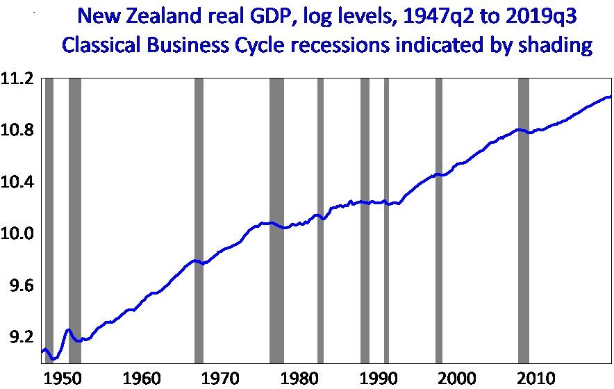
]]>Unfortunately, official New Zealand data on quarterly GDP does not go back very far in time, limiting our ability to understand recessions and expansions. Here I want to share some work I’ve done trying to build a consistent GDP series for New Zealand that goes back until 1947.
To extend New Zealand GDP figures beyond the time horizon given by official estimates Hall and McDermott (2011) used a range of econometric methods to estimate a quarterly GDP series using annual GDP data and quarterly indicators of the economy. The quarterly estimates developed by Hall and McDermott (2011) go all the way back to 1947 providing many more episodes of recession to study than would have been the case had we used only official data, learn about why getting a virtual reception for your business is a great option for growth.
The data can be found at the following link.
Figure 1 plots the natural logarithm of real GDP since 1947 for New Zealand with key New Zealand recessions shaded in grey. Over these 70 plus years the size of the economy has increased more than seven-fold. However, this growth has not followed a steady path. There have been periods of significant increases and declines in output and these variations makeup the New Zealand business cycle.
New Zealand’s Classical Real GDP Business Cycles: 1947 – 2019

There are a myriad of stories which come out of this data, such as:
- Why are there periods with much stronger trend growth (1950-1976) and much weaker trend growth (1976-1991)?
- What were the reasons for each of the recessions (contractionary phases) listed above?
- At 42 quarters, the current expansionary phase is the second longest on record – although with lower average growth than many other phases. What does this mean?
If there are any particular items you’d like discussed in the future, I’d be keen to hear your thoughts.
References
Hall, Viv B and C John McDermott, “A Quarterly post-Second World War Real GDP Series for New Zealand,” New Zealand Economic Papers, 45(3), December 2011, 273-298, Table A4.
Hall, Viv B and C John McDermott, “Recessions and Recoveries in New Zealand’s post-Second World War business cycles,” New Zealand Economic Papers, 50(3), December 2016, 261-280.
]]>In this post I am going to discuss the case for interest rate cuts during a natural disaster, to help to explain what demand shock they are battling and why this cut makes sense. The RBNZ already applied this logic during the Canterbury earthquake in 2011, so it is useful to think about COVID-19 from a similar perspective.
I’d like to thank the people I’ve chatted with about this issue to clarify what is going on – you know who you are, and I appreciate it. The New Zealand economics community is wonderful!
Background cuts
Central Banks around the world have already responded to COVID-19 with emergency interest rate cuts this month. The US has lowered their cash rate to 1.25% from 1.75%, Australia cut their rate to 0.5% from 1%.
New Zealand’s next decision on the OCR is on 25 March, where it’s highly expected that RBNZ will cut the rate by 0.5 bp – although this will depend on how they view the relative macro “demand” and “supply” factors.
Finding this balance is hard as I’ve discussed here and here. So it is useful to look at history to get some perspective. There are a multitude of events that might be useful for thinking through this process (September 11 attacks, SARS, the GFC) but I think the best is the Canterbury earthquakes – both in terms of how this is similar, and how this is different.
Do we need to cut the OCR to respond to the COVID-19?
As I have noted in my previous posts on COVID-19, the central bank is the main agency that must deal with a demand shock caused by the outbreak. Cutting the OCR is the natural monetary policy response to deal with the shock, preventing economic growth from slowing below its potential and keeping inflation rate within the target band.
In this way, COVID-19 is, in many ways, nothing like the Canterbury earthquake. There is a reduction in demand for NZ goods and services due to the pandemic occurring overseas (a decline in the price received for exports), and if it arrives onshore there is a “supply” shock due to people needing to stay at home instead of working.
Let’s think about this external demand shock more carefully.
Everyone is talking about supply chain disruption as if it is a supply shock. But although this is for the world in reality, this is the external demand shock for a place like New Zealand.
New Zealand is largely a primary goods producer, so such disruption is more of a demand shock – it lowers the price we receive for goods and services we sell, rather than increasing the price of intermediate inputs. In fact, with collapsing oil prices the “intermediate” price channel (the supply shock) doesn’t really seem relevant and we have to be careful not to start using this idea as a reason not to do appropriate demand management.
But if this external demand shock is the only shock, it may not be too necessary to stimulate demand – as it isn’t clear export prices have fallen off a cliff. Yes tourism operators are struggling, and forestry is having to hold logs, but the specific demand shock from the export sector may have already been more than made up for by the drop in the exchange rate already – suggesting this is more an issue of business continuity (helping illiquid but solvent providers stay afloat during a shock) than demand management.
But there are more channels.
With stock prices falling and uncertainty measures surging there may be a concern that banks will stop lending – this is another very important issue, the financial channel that was so important in the GFC. But this doesn’t necessarily mean cutting interest rates – instead the Bank can respond by loosening its macroprudential regulations and providing liquidity with unconventional tools.
So why do I still think a cut is appropriate? Let’s go back to the Canterbury earthquakes. There was no drop in external demand, no financial constraints, but there was a panic which lowered consumer and business confidence and negatively affected “animal spirits”. The Bank responded to this then by cutting interest rates – that was the right call then, and the right call now.
We don’t need fancy arguments to justify a cut, when a sharp drop in domestic demand due to fear of a pandemic already indicates that a cut is appropriate.